Lagrange Interpolation in MATLAB

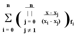
Named after Joseph Louis Lagrange, Lagrange Interpolation is a popular technique of numerical analysis for interpolation of polynomials. In a set of distinct point and numbers x_j and y_j respectively, this method is the polynomial of the least degree at each x_j by assuming corresponding value at y_j. Lagrange Polynomial Interpolation is useful in Newton-Cotes Method of numerical integration and in Shamir’s secret sharing scheme in Cryptography.

In this tutorial, we’re going to write a program for Lagrange Interpolation in MATLAB, and go through its mathematical derivation along with a numerical example. You can also check out our earlier tutorial where we discussed a C program for this interpolation technique.

Derivation of Lagrange Interpolation:

Consider a given set of k+1 points, (x₀, y₀) , (x₁, y₁), ( x₂, y₂)….. (x_k, y_k) where each points are distinct.

Let’s assume a function  L(x_j) such  that L(x_j) = y_j , j = 0, 1 , 3 , 3 . .. k

Observing the following points

• L_j(x) contains k factors in product and each factor has x
• 

Now, consider what happens when this product is expanded.

Since the product skips m = j, when i = j then all terms are [x_j – x_m ] / [x_j – x_m] =1

Also, when i ≠ j, m ≠ j does not produce it and one term in the product will be for m = I, that is, [x_i – x_i]/[x_j – x_i] = 0

Zeroing the entire product,

where, δ_ij is Kronecker’s delta.

So, it can be written that:

Therefore, the considered function L(x) is a polynomial with degree at most k and where L(x_j) = y_j

So, for all i ≠ j, l_j(x) includes the term ( x – x_i ) in the numerator, therefore the entire product will be found to be zero at x = x_j

This is the required formula which will also be used in the program code for Lagrange Interpolation in MATLAB.

NOTE:

The Lagrange Interpolation formula can also be derived from Newton’s divided difference formula.

When a polynomial function f(x) is be approximated with an n^th degree polynomial, nth divided difference of f(x) is constant and the (n+1)^th divided difference is zero.

Mathematically, f[x₀, x₁, x₂, x₃, . . .  . .  ..  . x_n] = 0

By using the second property of divided difference, it can be written that

Simplifying this equation, we get

This can be represented as:

Lagrange Interpolation in MATLAB Code:

% Lagrange Interpolation MATLAB Program
function [P,R,S] = lagrangepoly(X,Y,XX)
X = [1 2 3 4 5 6 7 8]; % inputting the values of given x
Y = [0 1 0 1 0 1 0 1]; % inputting the values of given y
%[P,R,S] = lagrangepoly(X,Y);
xx = 0.5 : 0.01 : 8.5; 
%plot(xx,polyval(P,xx),X,Y,'or',R,S,'.b',xx,spline(X,Y,xx),'--g')
%grid
%axis([0.5 8.5 -5 5])
if size(X,1) > 1;  X = X'; end % checking for parameters 
if size(Y,1) > 1;  Y = Y'; end
if size(X,1) > 1 || size(Y,1) > 1 || size(X,2) ~= size(Y,2)
  error('both inputs must be equal-length vectors') % displaying error
end % end of scope of if
N = length(X);
pvals = zeros(N,N);
% for evaluating  the polynomial weights for each order
for i = 1:N
  % the polynomial with roots may be values of X other than this one
  pp = poly(X( (1:N) ~= i));
  pvals(i,:) = pp ./ polyval(pp, X(i));
end
P = Y*pvals;
if nargin==3
  YY = polyval(P,XX); % output is YY with given XX
  P = YY; % assigning to output
end
% end of scope of if 
if nargout > 1 % checking for conndtions 
  R = roots( ((N-1):-1:1) .* P(1:(N-1)) );
  if nargout > 2
    % the evalustion of acual value at  the poins of zero derivative  
    S = polyval(P,R);
  end
end

The above Matlab code for Lagrange method is written for interpolation of polynomials fitting a set of points. The program uses a user-defined function named LAGRANGE(X, Y) with two input parameters which are required to be row vectors.

The row vectors X and Y define a set of n points which are used in Lagrange method for the determination of (n-1)^th order polynomial in X which passes through these points.  The function of P in the program is to return the n coefficients which define the polynomial in the same order as used by POLY and POLYVAL.

Similarly, R and S are defined to return x-coordinates and y-values at n-1 extreme of the resulting polynomial. YY returns the value of the polynomial sampled at the points which are specified in XX.

All the inputs which are required to give to the program are embedded in the source code. The values of X and Y initially set in the program are:

X = [1 2 3 4 5 6 7 8] and Y = [0 1 0 1 0 1 0 1]

A sample output of this MATLAB program is given below:

Numerical Example in Lagrange Interpolation:

Now, let’s analyze Lagrange Interpolation and its Matlab code mathematically using a different set of parameters. The question here is:

From  the following sets of data, find the value of x corresponding to y=15 by using Lagrange Interpolation.

(5,12), (6,13), (9,14),  11,16)

Solution

Given value of x and y are:

X: 5    6    9    11

Y: 12  13  14  16

By using the Lagrange Interpolation Formula:

x(y)=(y-13)(y-14)(y-16)*5/(12-13)(12-14)(12-16) + (y-12)(y-14)(y-16)*6/(13-12)(13-14)(13-16) + (y-12)(y-13)(y-16)*9/(14-12)(14-13)(14-16) + (y-12)(y-13)(y-14)*11/(16-12)(16-13)(16-14)

By substituting y= 15, we get x = 11.5; which is the required answer.

If you have any questions regarding Lagrange interpolation, its MATLAB code, or its derivation, bring them up to us from the comments section. You can find more Numerical methods tutorial using Matlab here.